Plotting species introductions between continents
Source:vignettes/plotting_introductions.Rmd
plotting_introductions.RmdHere in this article, we show how to use the package’s function
introGraph to plot where the species of any plant family or
genus were introduced from and to. The graphic is a heatmap with the
number of species native to each continent (rows) that are introduced in
each other continent (columns), following the World Geographical Scheme
for Recording Plant Distributions. It helps to see which floras are
the main sources of introduced plants, and which continents receive most
of them.
Setup
Install the latest development version of expowo from GitHub:
#install.packages("devtools")
devtools::install_github("DBOSlab/expowo")1. Mining the species list and their distribution
introGraph uses as input data the species list and their
native and introduced distribution returned by powoSpecies.
The first search downloads the data of the World Checklist of Vascular
Plants (about 90 MB) only once, so any following search takes a few
seconds.
fab <- powoSpecies(family = "Fabaceae",
                   verbose = FALSE)
2. Plotting introductions between continents
Just provide the output of powoSpecies to
introGraph. Each botanical country of the native and
introduced distribution of each species is assigned to its continent,
and a species counts once for each pair of continents. Introductions
within the same continent are not shown. No download is needed, as the
continent of each botanical country is stored within
expowo. Setting save = TRUE writes the
graphic within a subfolder named after the current date, in any of the
formats JPG, PDF, PNG or TIFF.
introGraph(inputdf = fab,
           save = TRUE,
           dir = "results_introGraph",
           filename = "intro_graph_Fabaceae",
           format = "png")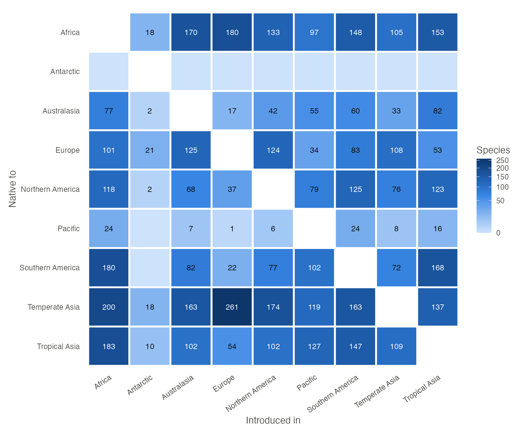
FIGURE 1. Number of Fabaceae species native to each continent (rows) that are introduced in each other continent (columns).
About 1,300 legume species are introduced in another continent.
Species native to temperate Asia, i.e. the Mediterranean and western
Asian clovers, medicks and vetches, are the most widely introduced,
above all in Europe, Africa and Northern America. Africa and tropical
Asia are also major sources of introduced legumes. The Antarctic
continent of the scheme includes the subantarctic islands, where some
legumes were introduced.
3. Plotting introductions between regions
For a finer view, the argument level = "region" uses the
52 regions of the level 2 of the scheme (e.g. Brazil, Southwestern
Europe, Indo-China) instead of the nine continents. The graphic is
larger, and it is saved with a larger size accordingly.
introGraph(inputdf = fab,
           level = "region",
           save = TRUE,
           dir = "results_introGraph",
           filename = "intro_graph_Fabaceae_regions",
           format = "pdf")
4. Using the graphic object
introGraph returns a ggplot object, so the
graphic can be customised with any function of ggplot2.
The data of the graphic has the number of species (species)
native to each continent or region (from) that are
introduced in another one (to).
p <- introGraph(fab, verbose = FALSE)

# Main routes of introduction
routes <- p$data[order(-p$data$species), c("from", "to", "species")]
head(routes)

# Adding a title
p + ggplot2::ggtitle("Where legumes were introduced")
When the input data has synonyms (a status column, as in
powoSpecies(synonyms = TRUE)), only accepted species are
counted.